In the last article of this series we talked about generation of a test set and also the different ways in which we can generate it (i.e. Random sampling, Stratified sampling).

Once we have separated our dataset into training set and test set we will not look at our test set until we have finished training our model with the training set.

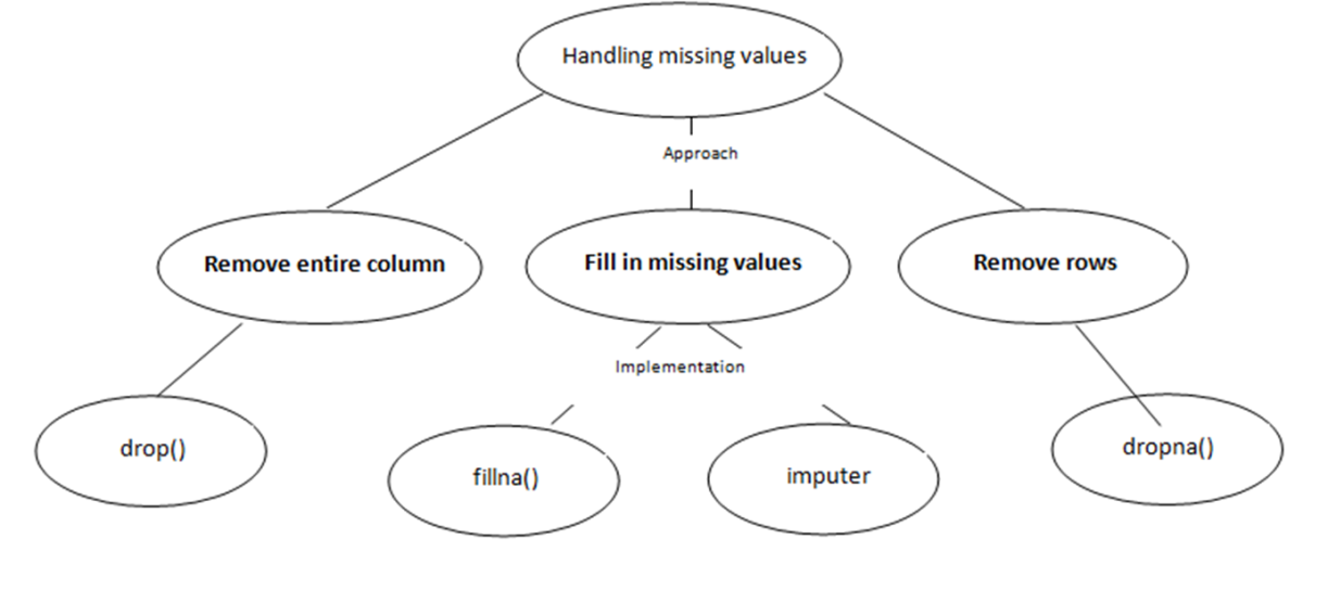
Handling missing values

Most of the times the data in the training set would have missing values for some of the columns. “Most machine learning algorithms cannot work with missing values in its input features”.

There are typically three ways of handling missing data

Let’s look at a sample dataset. This dataset was downloaded from Kaggle (https://www.kaggle.com/fernandol/countries-of-the-world/data)and contains the population, area and other information about the countries of the world. It contains 227 entries.

Let’s say we want to analyze the Infant Mortality rate.

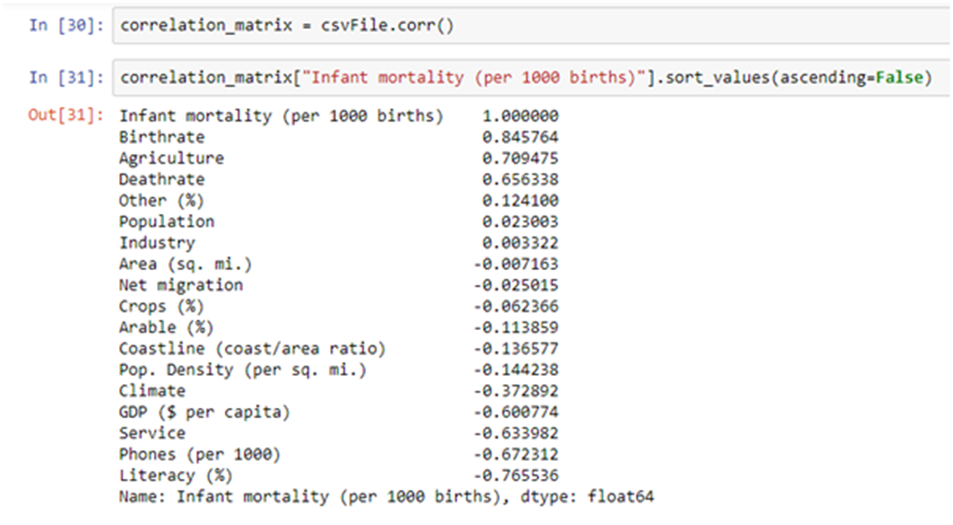
Let’s create the correlation matrix for ‘Infant mortality (per 1000 births)

Approach 1:- Remove columns

As you can see that the Birthrate, Agriculture and Deathrate have strong positive correlation whereas the GDP ($ per capita), Service, Phones (per 1000), Literacy (%) have a strong negative correlation.

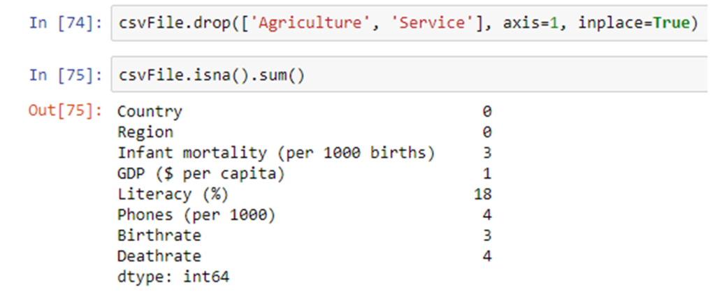
Let’s drop the columns, which have no correlation, from our dataset. We can do so by using drop() function.

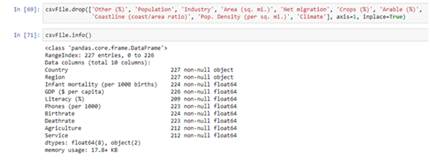
Next, Let’s check the number of entries, which contains Nan, in each of the columns

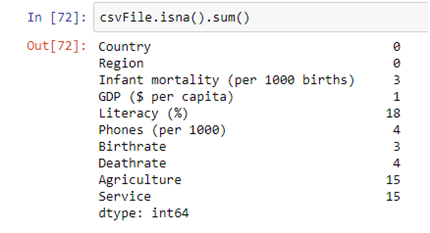
As you can see the Agriculture, Service and Literacy columns have many entries with null values.Let’s say we want to drop Agriculture and Service columns

Disadvantages of this approach:-

a. We may end up removing an important feature.

Approach 2:- Remove rows

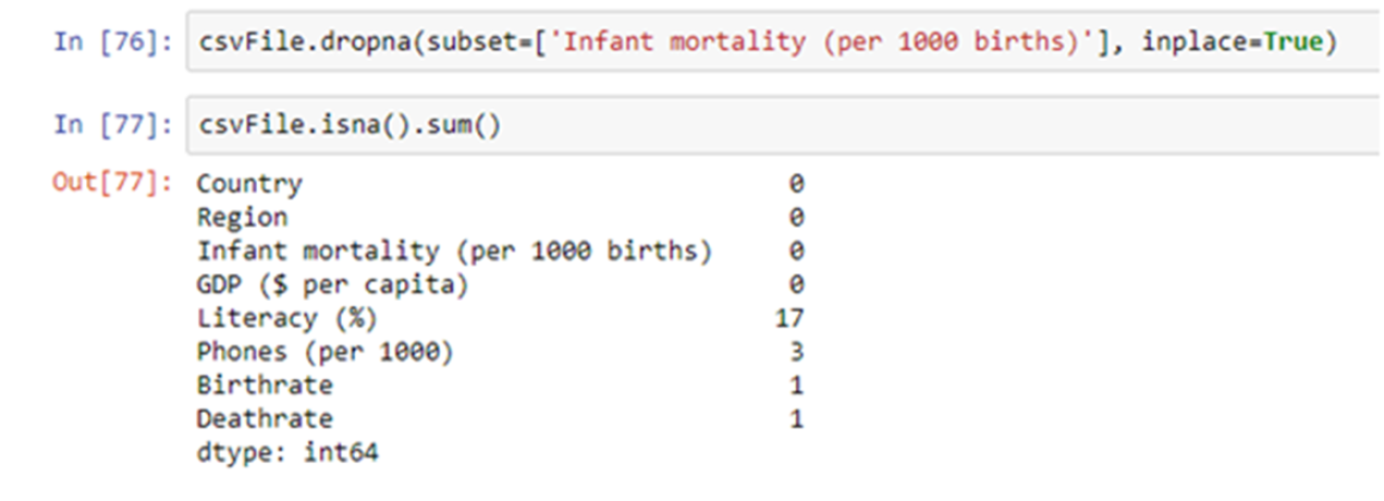
The Infant mortality column contains 3 null values. Let’s remove those rows. We can remove rows containing null values in a particular column using dropna() method.

Disadvantages of this approach:-

a. We may end up reducing the size of our training set by a significant number. Also there is a possibility that some important entries that we wish to have in our training set will be removed.

b)There is also a likely chance that an entire stratum will get removed or in the worst case scenario many strata will get removed. We may also end up reducing a significant number of entries from some of our strata, which might make the strata underrepresented in our training set. This can eventually result in our model not learning enough about those strata.

Approach 3:- Fill missing values

3.1 Using fillna() method

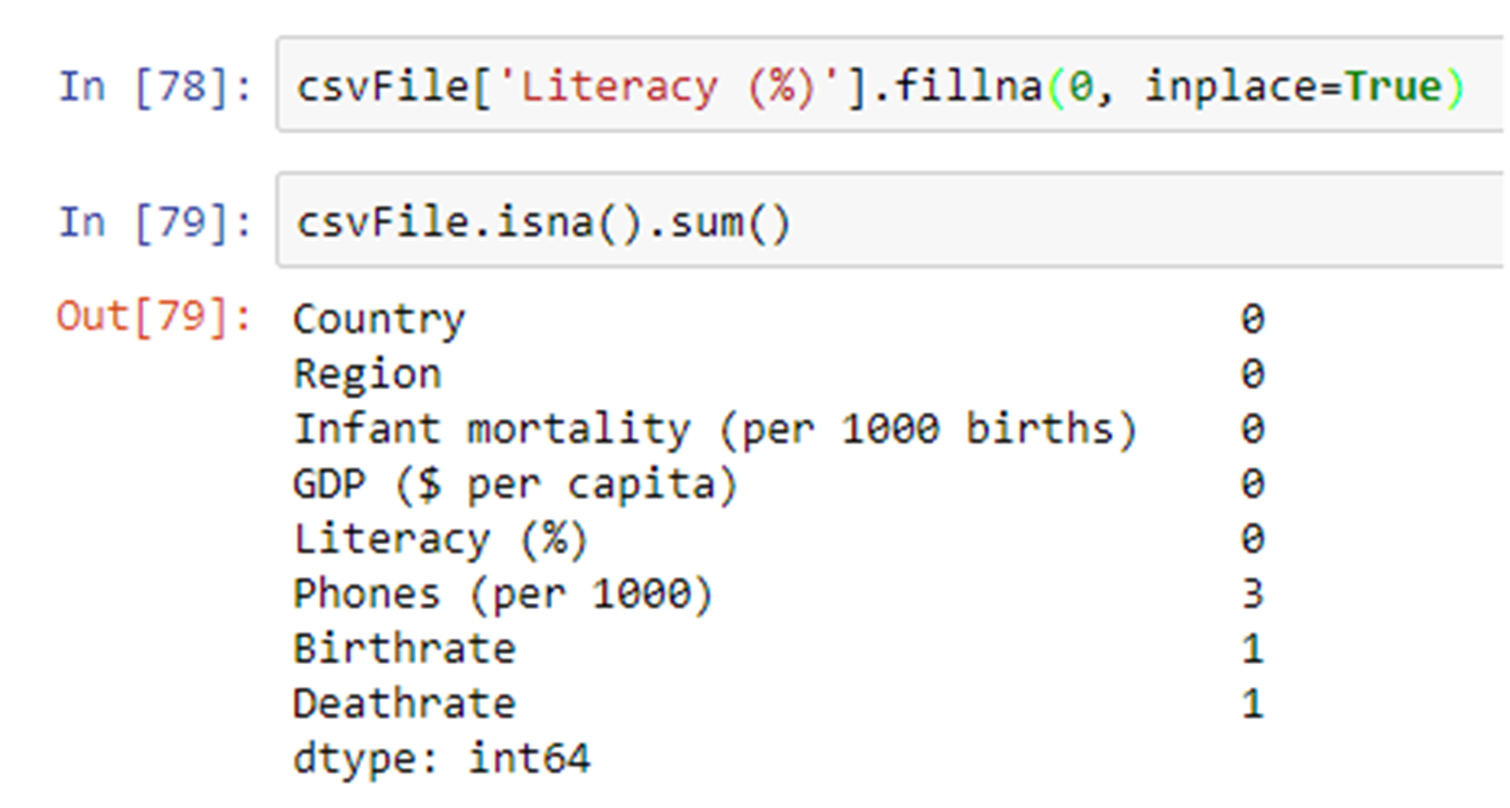
Let’s fill the null values in Literacy (%) column with 0 using fillna() method.

3.2 Using imputer

The second approach for filling missing values is to use an imputer. An imputer is a class provided by scikit for filling missing values.

An imputer estimates the mean or median or most frequent value depending on the imputer’s strategy. The imputer’s strategy is passed in its constructor as a parameter. The default value of the strategy parameter of the imputer is “mean”.

E.g. imputer = new Imputer(strategy = “median”).

An imputer can only work on numeric attributes.

Let’s say you want the imputer to compute the mean and fill the missing values.

Since the imputer can only work with numeric values, we will have to separate the numeric and string attributes.

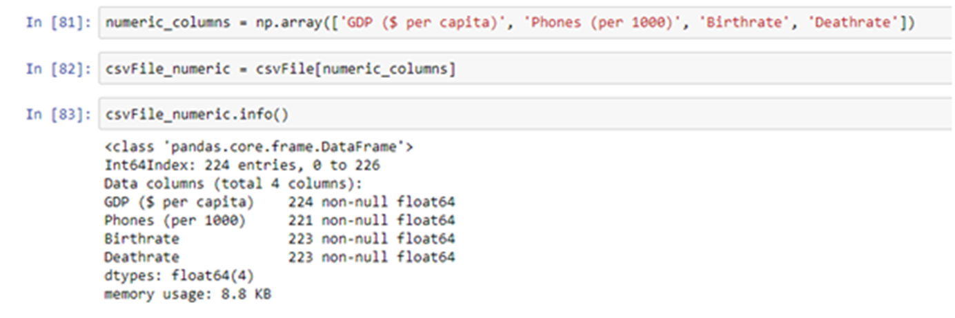
Note that we have not included the Literacy (%) because we had already used fillna() to fill missing values in it.

Let us now apply the imputer. We are not passing any strategy, hence the default strategy i.e. mean will be applied.

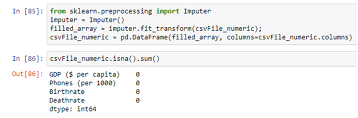
Handling string attributes

“ ML algorithms work well with numerical attributes”. So if you have any string attributes then you must convert it to numeric. In order to convert categorical string attributes to numbers scikit provides the LabelEncoder transformer.

Let’s encode the Region attribute.

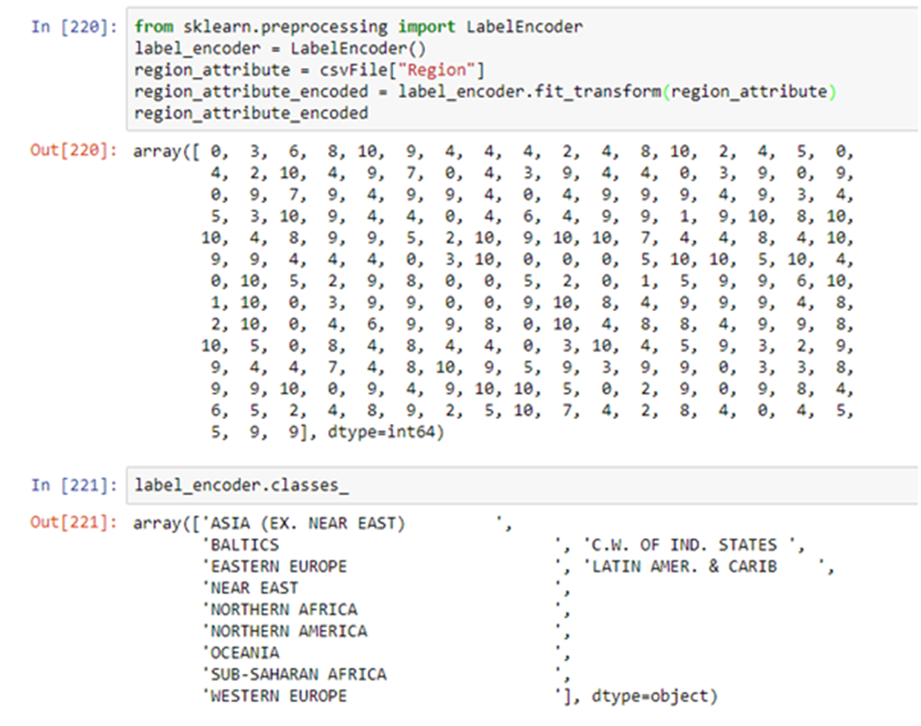
As you can see the label encoder has encoded the Region column with numbers. The LabelEncoder associates each class with a number(label) i.e. ‘ASIA (EX. NEAR EAST)’ has been assigned label 0, ‘BALTICS’ has been assigned label 1, and so on.

The only issue with assigning labels is that some ML algorithms will assume that two nearby values are more related than two distant values. For e.g. ML algorithm may assume that ‘Eastern Europe’(label 3) is more similar to ‘Latin Amer. & Carib’(label 4) and less similar to ‘Western Europe’(label 10).

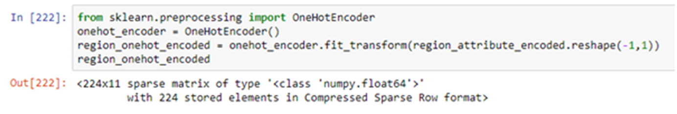
In order to resolve this problem scikit provides an encoder called OneHotEncoder. OneHotEncoder converts the categorical values to one-hot vectors. But the categorical values must be of type integer.

Let’s one hot encode the label encoded regions.

If you wish to perform both LabelEncoding and OneHotEncoding in one shot, there are two approaches:-

1) Use the LabelBinarizer class of scikitlearn

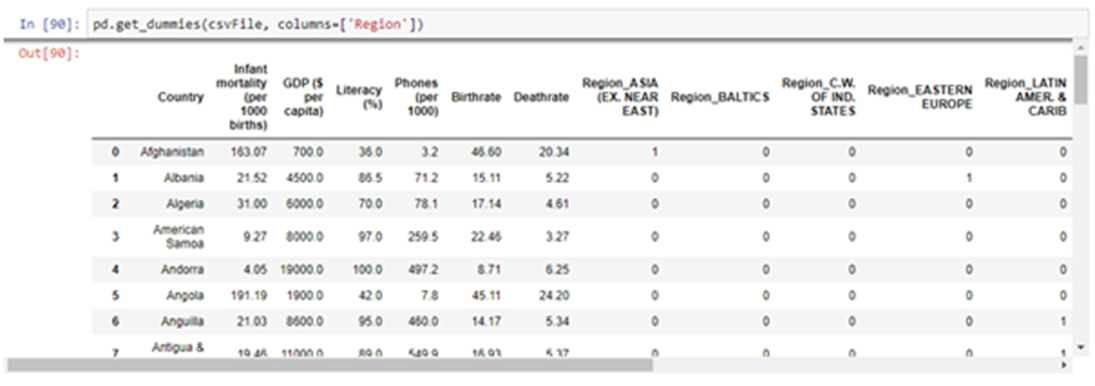
2) Use the get_dummies() function of pandas.

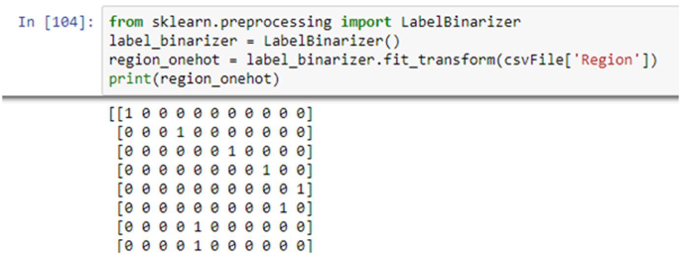
The only difference between them is that LabelBinarizer will take one column and return a numpy array containing one hot encoded values whereas the get_dummies() takes the entire dataframe and returns a dataframe which will contain one hot encoded columns along with other columns. The get_dummies() method has a parameter named columns which takes a list of columns that you wish to encode

Approach 1:- Use the LabelBinarizer class of scikitlearn

Approach 2:- Use the get_dummies() function of pandas.

So far we have performed many transformations on our training set. After we have trained our model we would like to test our performance on our test set. At that time we will have to apply the transformations in the exact same sequence that we have applied on training set, on the test set and then perform our predictions.

For this we will have to maintain the sequence of the transformations i.e first we applied fillna() on “Literacy (%)” column, then applied imputer on the numeric columns, then one hot encoded the Region column etc

Scikit-learn provides the Pipeline class to create a sequence of transformations. We would create a pipeline of transformations only once and it can then be used on training set, test set and future samples. We will explain Pipelines in depth in the next blog.

Until next time!

Team Cennest